Computer Concepts in Action ©2009

Unit 5: Spreadsheets

Use Multiple Criteria Sorts in Excel

In Excel you can sort data by specific column or by multiple columns. Using this feature you can quickly and easily alphabetize names or put numbers in order.

Once the data on your worksheet is complete, you may want to change the way the worksheet looks. Formatting can give a worksheet a distinct style or make data easier to read. You can use the Styles feature to apply pre-existing formats to a worksheet.

To open the data file in Step 1, click on the link. If you are not able to download the file, ask your teacher for help.

1. Start Microsoft Excel, then open your Allowance file. (Note: If you did not complete Enrichment Activity 5.1, use the Allowance (7.0K) data file for this activity.)



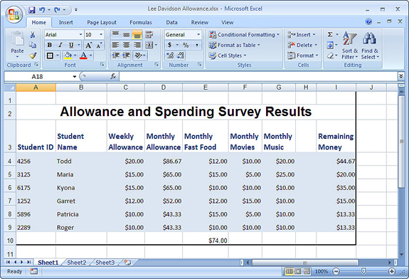
2. Click cell B4. Drag the pointer to cell I9 and release (see Figure 1).

Figure 1: Select cells B4 through 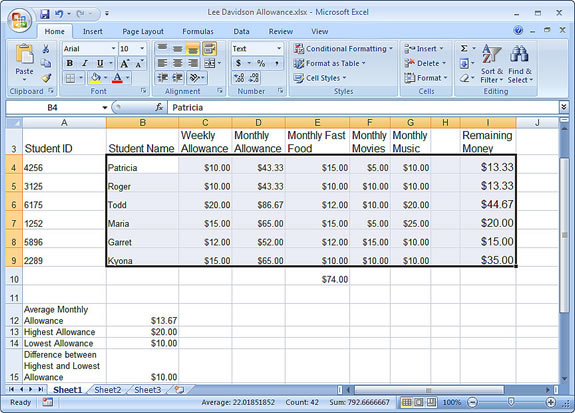<a onClick="window.open('/olcweb/cgi/pluginpop.cgi?it=jpg::::/sites/dl/free/0078805775/595819/EnrichmentAct5_2_U05_SC01.jpg','popWin', 'width=NaN,height=NaN,resizable,scrollbars');" href="#"><img valign="absmiddle" height="16" width="16" border="0" src="/olcweb/styles/shared/linkicons/image.gif"> (72.0K)</a>

3. Click the Home tab, and then click the Sort & Filter button. Click Custom Sort. The Sort dialog box opens (see Figure 2).



4. Use the Sort by arrow to choose Column D.



5. Click Largest to Smallest in the Order section.



6. Click the Add Level button. Use the Then by arrow to choose Column E.



7. Click Largest to Smallest in the Order section (see Figure 2).

Figure 2: The Sort box lets you sort multiple columns in Excel. 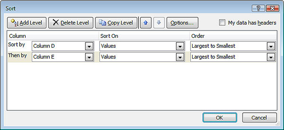<a onClick="window.open('/olcweb/cgi/pluginpop.cgi?it=jpg::::/sites/dl/free/0078805775/595819/EnrichmentAct5_2_U05_SC02.jpg','popWin', 'width=NaN,height=NaN,resizable,scrollbars');" href="#"><img valign="absmiddle" height="16" width="16" border="0" src="/olcweb/styles/shared/linkicons/image.gif"> (101.0K)</a>

8. Click OK. Deselect the cells by clicking outside the area.



9. The cells have been rearranged to arrange the monthly allowance from highest to lowest. Then, for each allowance amount, the largest amount spent on fast food is displayed first (see Figure 3).

Figure 3: The final worksheet 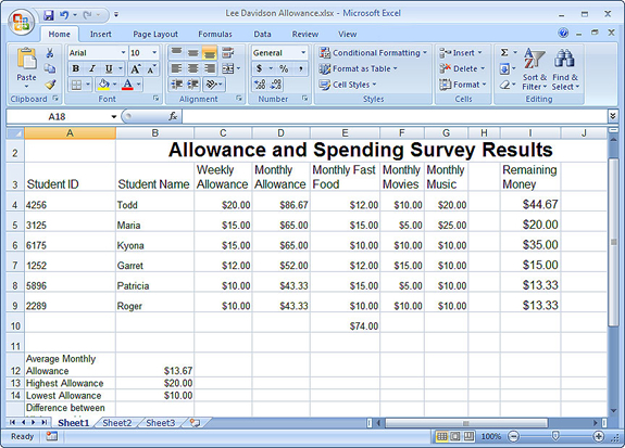<a onClick="window.open('/olcweb/cgi/pluginpop.cgi?it=jpg::::/sites/dl/free/0078805775/595819/EnrichmentAct5_2_U05_SC03.jpg','popWin', 'width=NaN,height=NaN,resizable,scrollbars');" href="#"><img valign="absmiddle" height="16" width="16" border="0" src="/olcweb/styles/shared/linkicons/image.gif"> (285.0K)</a>

10. Select cells A3:I3. Click the Home tab, then click the Cell Styles button. Click the Heading 2 style.



11. Select cells A4:I9, and click the Cell Styles button. Click one of the 20% - Accent 1 buttons.



12. Select cells A1:I10. Click the arrow beside the Border button, and click Thick Box Border.

Figure 4: The formatted worksheet <a onClick="window.open('/olcweb/cgi/pluginpop.cgi?it=jpg::::/sites/dl/free/0078805775/595819/EnrichmentAct5_2_U05_SC04.jpg','popWin', 'width=NaN,height=NaN,resizable,scrollbars');" href="#"><img valign="absmiddle" height="16" width="16" border="0" src="/olcweb/styles/shared/linkicons/image.gif"> (265.0K)</a>

13. Save and close your Allowance file.



14. Exit Excel.