Computer Concepts in Action

Unit 5: Spreadsheets

Work with More Worksheet Formulas and Functions

Work with More Worksheet Formulas and Functions – Part 1

Insert a Function into a Formula

Formulas in Excel can contain several different kinds of values, including numbers, references to other cells, mathematical operators like + (addition) and * (multiplication), and functions like AVERAGE and COUNT. When several operations and functions are combined into a single formula, Excel performs the operation in the following order, or precedence:

( ) Parenthesis
: Reference Operator
% Percent
^ Exponent
* and / Multiplication and Division (from left to right)
+ and - Addition and Subtraction (from left to right)

The order in which Excel calculates a formula can be changed by enclosing the part of the formula to be calculated first in parenthesis.

A Worksheet Function (SUM, AVERAGE, COUNT, etc.) is a built-in mathematical formula that makes it easier for you to accomplish tasks when working with large worksheets. Worksheet formulas often include one or more functions. In the next exercise, you will be using a data file to find out how much allowance money a student has left after her expenses. The worksheet already contains some functions, and you will be adding your own.

To open the data file in Step 1, click on the link. If you are not able to download the file, ask your teacher for help.

Start Microsoft Excel.
Open the data file Allowance (17.0K) .
Save the file as Your Name Allowance.
Select cell I4 in the Remaining Money column.
Press the = key to start a new function.
Select cell D4, and then press the – key.
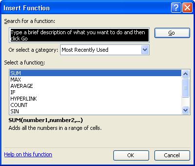
To add a function to the formula, click the Insert menu, then choose Function. The Insert Function box opens (see Figure 1).

Figure 1 The Insert Function box
Select SUM and click the OK button (you may need to select All in the Or select a category drop-down list and scroll down to find the function).
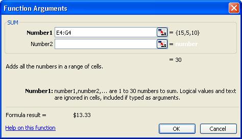
The Function Arguments box opens.
In the Number 1 field, type the range E4:G4 (see Figure 2).

Figure 2 The Function Arguments box
Click the OK button. You have now added the cells that display Patricia’s monthly expenses. These are then subtracted from her monthly allowance.
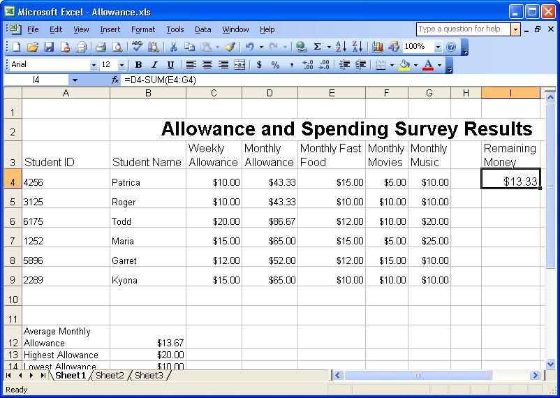
The amount of money Patricia has remaining after her expenses appears in cell I4 (see Figure 3).

Figure 3 The formula has been applied to cell I4.
Repeat steps 2 through 9, using the appropriate cells to find the Remaining Money amounts for the rest of the students.
Save your file.

Work with More Worksheet Formulas and Functions – Part 2

Add a Second Function to a Formula

In the previous activity, you created formulas that used a single function to determine the amount of money that students had after monthly expenses. You can also use multiple functions in a formula to calculate additional information. In this exercise you will calculate the difference between the highest and lowest allowances in the worksheet.

In your Allowance file, select cell B15 (you may need to scroll down).
Click the Insert Function button to start a new formula. The Insert Function box opens.
Select MAX and click the OK button (Note: You may need to scroll through the Or select a category list and select All.)
In the Function Arguments box, type the range C4:C9 in the Number 1 field.
Click the OK button. The highest weekly allowance appears in cell B15.
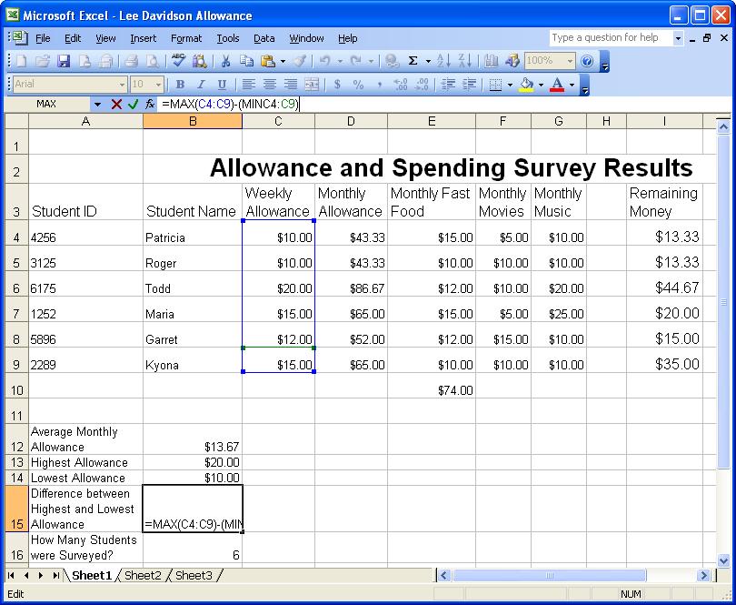
In the formula bar, place your insertion point at the end of the displayed function. Then press the – key (see Figure 4).

Figure 4 Add a second function.
Type MIN to start the second function in the formula.
Type (C4:C9). The displayed formula shows the minimum allowance in Column C subtracted from the maximum allowance.
Press the Enter key. The difference between the highest and lowest weekly allowances appears in cell B15 (see Figure 5).

Figure 5 The formula is applied to cell B15.
Save your file.

Work with More Worksheet Formulas and Functions – Part 3

Fix an Error in a Formula

On occasion, a change in information or a minor mistake will make it necessary to edit or revise a formula or function. For example, you might accidentally try to apply a formula to cells that contain only text. Perhaps a date, dollar amount, or cell reference range has been typed in incorrectly.

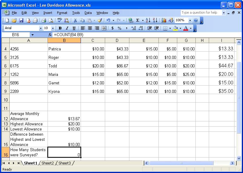
To fix a formula, you can simply click on the cell in which the formula is contained, move the curser to the formula bar, highlight the error or data to be changed, and replace it with the correct data.

In your Allowance file, select cell B16.
Look at the formula bar. The cell range used for the COUNT function is for Student Name (B4 through B9), which in this instance is incorrect. The COUNT function adds up the number of cells which contain numbers (or a written number, like “one”). If the text cannot be translated into a number it is ignored. Therefore, the COUNT function should be applied to Student ID (A4 through A9).
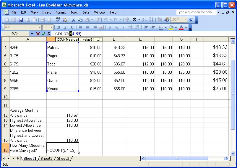
In the Formula Bar, select the first letter B (see Figure 6).

Figure 6 Apply the COUNT function to the Student ID range of cells.
Type the letter A.
Select the second letter B.
Type the letter A again.
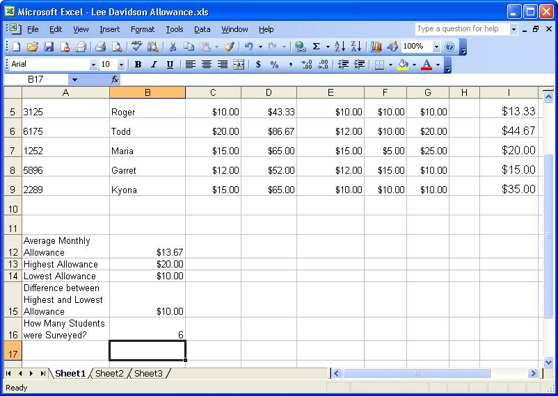
Press the Enter key.
The total number of students appears in cell B16 (see Figure 7).

Figure 7 The COUNT function adds up the students.
Save your file.

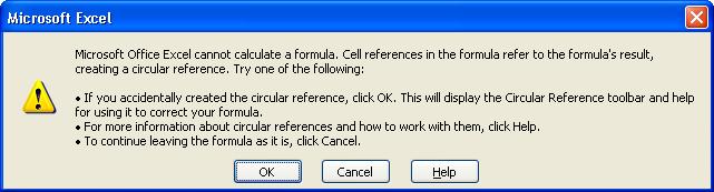
Work with More Worksheet Formulas and Functions – Part 4

Correct a Circular Reference

When using formulas and functions, errors like the one in the previous exercise are common, and that is why it is very important to enter data carefully and check your work. Circular references (entering a formula that references the same cell that contains the formula being created) are another common type of error.

In your Allowance file, select cell E10.
Type =SUM(E4:E10) in the formula bar.
Press the Enter key.
Read the circular reference notification that appears (see Figure 8).

Figure 8 The circular reference notification
Click the Cancel button on the error message to continue (click OK for more information on circular references).
Select cell E10 again.
Select the number 10 in the formula bar and type the number 9.
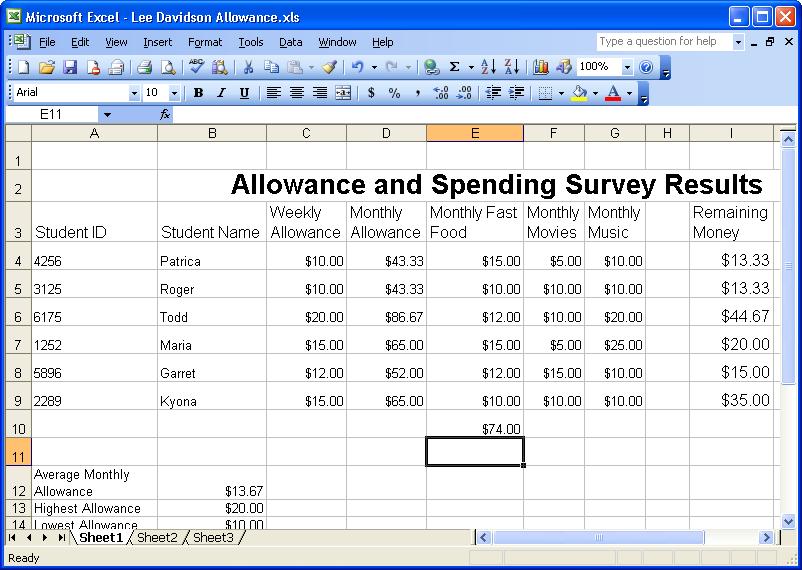
Press the Enter key. The total amount spent by all the students on fast food in a month appears in cell E10 (see Figure 9).

Figure 9 The circular reference has been corrected.
Save and close your Allowance file.
Exit Excel

Search
Search for:

Site Preferences	(Log out)

		Send mail as:

TA email:
Other email:

"Floating" navigation?
Drawer speed:

Teacher Log In
Log in here to access teaching material for this site.
Username:
Password:

Home > > Unit 5 > Enrichment Activity 5.1
Computer Education Home Product Info Site Map Contact Us